So it has been a while since I last dropped out a blog, but this one was useful to me at work, so I thought I would share.
Office 2016 (or 2013 and 365) has some lovely functions, one of them being conditional formatting. I use this quite a lot, but one thing stumped me. Below is what I wanted to get to:
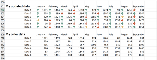
When I wanted to compare to tables of data and put in place icons to show if the data had moved up or down, I could not do it. Excel would politely tell me that “This type of reference cannot be used in a Conditional Formatting formula”

Now, not being one to like these limitations, I realised that I could do it cell by cell, but that would be an awful lots of mouse clicks, so I’ve written this short piece of VBA to do it for you. To open the VBA environment, press-Alt-F11 then right click your VBAProject and select Insert Module. You can then paste the code from below into that window and modify the CompareIcons sub to match your needs. The “CompareIcons” sub makes a call GenericIconsComparison which implements the conditional formatting. The parameters are:
| Parameter |
Description of use |
| IconsTopleft As Range, |
This is the location of the top left corner of the cells where your icons will appear. It can also be the complete range of cells that you want to put in comparison icons |
| CompareTopLeft As Range, |
This is the top left location of the cells that you are comparing to |
| Rows As Integer, |
If you only entered a single cell for the IconsTopLeft parameter, then you can enter the number of rows here |
| Cols As Integer, |
If you only entered a single cell for the IconsTopLeft parameter, then you can enter the number of Columns here |
| Icons As XlIconSet, |
Within Excel there are a number of icons, I used xl3Arrows |
| ReverseOrder As Boolean, |
If you wish to make it that higher values are red and lower valued are green, put True here, otherwise put in False |
| ShowIconsOnly As Boolean, |
If you want to hide the values in the cells and only show icons, put True here, otherwise put False |
| RemoveOtherCondFormatting As Boolean |
If you want to remove any other Conditional Formatting, including previous use of this command, set this to True |
The code – first a sample macro to call the routine to deliver the comparison icons
Sub CompareIcons()
'In this example it starts in cell Q202 and compares to the cell Q210 and does this for 5 rows and 9 columns. The icons used at xl3Arrows and removes all other conditional formatting on the cells impacted.
Call GenericIconComparison(Range("q202"), Range("q210"), 5, 9, xl3Arrows, False, False, True)
'In this example it compares the range from Q202:Y206 to the cells starting in Q210, so in effect the same as the one above
Call GenericIconComparison(Range("q202:Y206"), Range("q210"), 0, 0, xl3Arrows, False, False, True)
'In this example it does the same as the others, except higher values get a downward arrow and lover values get a higher value
Call GenericIconComparison(Range("q210"), Range("q202"), 5, 9, xl3Arrows, True, False, True)
End Sub
Below is the VBA code to implement everything I’ve spoken about. It does what is says on the tin.
Sub GenericIconComparison(IconsTopleft As Range, CompareTopLeft As Range, Rows As Integer, Cols As Integer, Icons As XlIconSet, ReverseOrder As Boolean, ShowIconsOnly As Boolean, RemoveOtherCondFormatting As Boolean)
'
' Icon Comparisons for ranges
'
'get column top left for from and too ranges
from_col_number = IconsTopleft.Column
to_col_number = CompareTopLeft.Column
'If a range is given, use that over rows and cols parameters
If IconsTopleft.Columns.Count > 1 Then Cols = IconsTopleft.Columns.Count
If IconsTopleft.Rows.Count > 1 Then Rows = IconsTopleft.Rows.Count
For i = 1 To Cols
'get Column letter for from cell
from_col = from_col_number + i - 1
If from_col > 26 Then
col = Chr(64 + Int((from_col - 1) / 26)) + Chr(64 + from_col - Int((from_col - 1) / 26) * 26)
Else
col = Chr(64 + from_col)
End If
'get Column letter for comparison cell
to_col = to_col_number + i - 1
If to_col > 26 Then
ToCol = Chr(64 + Int((to_col - 1) / 26)) + Chr(64 + to_col - Int((to_col - 1) / 26) * 26)
Else
ToCol = Chr(64 + to_col)
End If
'create the rules
For j = 1 To Rows
'select the cell
Range(col + Trim(j + IconsTopleft.Row - 1)).Select
'clear other formatting if desired
If RemoveOtherCondFormatting = True Then Selection.FormatConditions.Delete
'add the rule to compare to other cell
Selection.FormatConditions.AddIconSetCondition
Selection.FormatConditions(Selection.FormatConditions.Count).SetFirstPriority
With Selection.FormatConditions(1)
.ReverseOrder = ReverseOrder
.ShowIconOnly = ShowIconsOnly
.IconSet = ActiveWorkbook.IconSets(Icons)
End With
With Selection.FormatConditions(1).IconCriteria(2)
.Type = xlConditionValueNumber
.Value = "=$" + ToCol + "$" + Trim(j + CompareTopLeft.Row - 1)
.Operator = 7
End With
With Selection.FormatConditions(1).IconCriteria(3)
.Type = xlConditionValueNumber
.Value = "=$" + ToCol + "$" + Trim(j + CompareTopLeft.Row - 1)
.Operator = 5
End With
Next
Next
End Sub
blah
Posted
Sat, Feb 4 2017 12:56 AM
by
David Overton